Using derivative module

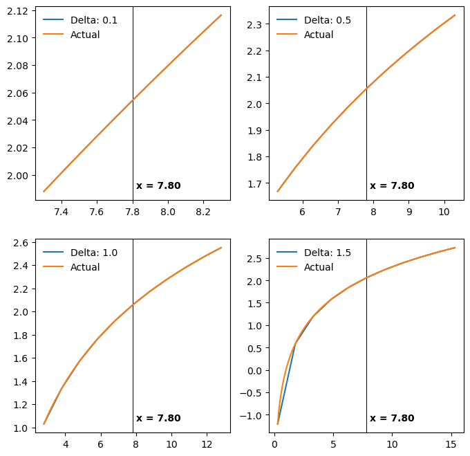
This contains a small script on how to perform multi-point first and second numercial derivates comparing them to the expected result. Here, we try to approximate the first and second derivatives of \(y = ln(x)\) with a displacement of 0.1, 0.5, 1.0, and 1.5. We then show the improvement of the numercial derivative as we start to include more data points to the derivative. We have implemented code to calculate the numerical derivative with two, four, six, and eight symmetric displacment points. For the second derivative there is an extra point as the data from the equilibrium position is required. We use \(y=ln(x)\) as it has a very simple analytical first and second derivative of \(1/x\) and \(-1/x^2\), respectively.

from vibrav.numerical.derivatives import (two_point_1d, four_point_1d, six_point_1d, eight_point_1d,
                                          two_point_2d, four_point_2d, six_point_2d, eight_point_2d)
import matplotlib.pyplot as plt
import numpy as np
import pandas as pd

def do_derivs(delta, base, steps, stdout=False, first=True):
    x = np.linspace(base-delta*steps/2,base+delta*steps/2,steps+1)
    y = np.log(x)
    y_plus = y[-int(steps/2):]
    y_minus = np.flip(y[:int(steps/2)])
    y_equil = y[int(steps/2)]
    if first:
        actual = 1/base
        d_eight = eight_point_1d(y_plus[:4], y_minus[:4], delta)
        d_six = six_point_1d(y_plus[:3], y_minus[:3], delta)
        d_four = four_point_1d(y_plus[:2], y_minus[:2], delta)
        d_two = two_point_1d(y_plus[:1], y_minus[:1], delta)
    else:
        actual = -1/base**2
        d_eight = eight_point_2d(y_plus[:4], y_minus[:4], y_equil, delta)
        d_six = six_point_2d(y_plus[:3], y_minus[:3], y_equil, delta)
        d_four = four_point_2d(y_plus[:2], y_minus[:2], y_equil, delta)
        d_two = two_point_2d(y_plus[:1], y_minus[:1], y_equil, delta)
    cols = ['actual', 'delta']+[x+'-point' for x in ['two', 'four', 'six', 'eight']]
    df = pd.Series([actual, delta, d_two, d_four, d_six, d_eight], index=cols)
    return df

def gen_plot(fig_num, deltas, base, steps):
    fig = plt.figure(fig_num, figsize=(8,8), dpi=100)
    for i, delta in enumerate(deltas):
        ax = fig.add_subplot(2, 2, i+1)
        x = np.linspace(base-delta*steps/2,base+delta*steps/2,steps+1)
        y = np.log(x)
        ax.axvline(base, color='k', linewidth=0.7)
        ax.plot(x, y, label="Delta: {:.1f}".format(delta))
        act_x = np.linspace(base-delta*steps/2,base+delta*steps/2,1000)
        act_y = np.log(act_x)
        ax.plot(act_x, act_y, label="Actual")
        ax.legend(frameon=False, loc='upper left')
        ax.text(0.52, 0.05, 'x = {:.2f}'.format(base), va='bottom', ha='left',
                transform=ax.transAxes, fontweight='bold')

Setting \(x=7.8\)

\begin{equation} \frac{d}{dx}~ln(7.8) = 0.128205 ~~~~~~~~ \frac{d^2}{dx^2}~ln(7.8) = -0.016437 \end{equation} ### Plots with the numerical vs. actual values

gen_plot(1, [0.1, 0.5, 1, 1.5], 7.8, 10)

Numerical first derivative for delta of 0.1, 0.5, 1.0, and 1.5

derivs_1d = []
for d, delta in enumerate([0.1, 0.5, 1, 1.5]):
    df = do_derivs(delta, base=7.8, steps=10)
    df['index'] = d
    derivs_1d.append(df)
derivs_1d = pd.concat(derivs_1d, axis=1).T
derivs_1d['index'] = derivs_1d['index'].astype(int)
derivs_1d

	actual	delta	two-point	four-point	six-point	eight-point	index
0	0.128205	0.1	0.128212	0.128205	0.128205	0.128205	0
1	0.128205	0.5	0.128381	0.128203	0.128205	0.128205	1
2	0.128205	1.0	0.128915	0.128176	0.128209	0.128204	2
3	0.128205	1.5	0.129822	0.128044	0.128258	0.128155	3

Numerical second derivative for delta of 0.1, 0.5, 1.0, and 1.5

derivs_2d = []
for d, delta in enumerate([0.1, 0.5, 1.0, 1.5]):
    df = do_derivs(delta, base=7.8, steps=10, first=False)
    df['index'] = d
    derivs_2d.append(df)
derivs_2d = pd.concat(derivs_2d, axis=1).T
derivs_2d['index'] = derivs_2d['index'].astype(int)
derivs_2d

	actual	delta	two-point	four-point	six-point	eight-point	index
0	-0.016437	0.1	-0.016438	-0.016437	-0.016437	-0.016437	0
1	-0.016437	0.5	-0.016470	-0.016436	-0.016437	-0.016437	1
2	-0.016437	1.0	-0.016573	-0.016430	-0.016437	-0.016436	2
3	-0.016437	1.5	-0.016748	-0.016402	-0.016449	-0.016425	3

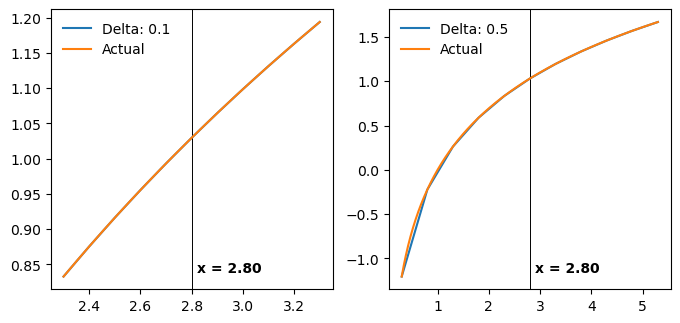
Setting \(x=2.51\)

\begin{equation} \frac{d}{dx}~ln(2.51) = 0.398406 ~~~~~~~~ \frac{d^2}{dx^2}~ln(2.51) = -0.158728 \end{equation} ### Plots with the numerical vs. actual values

gen_plot(2, [0.1, 0.5], 2.8, 10)

Numerical first derivative for delta of 0.1, and 0.5

derivs_1d = []
for d, delta in enumerate([0.1, 0.5]):
    df = do_derivs(delta, base=2.51, steps=10)
    df['index'] = d
    derivs_1d.append(df)
derivs_1d = pd.concat(derivs_1d, axis=1).T
derivs_1d['index'] = derivs_1d['index'].astype(int)
derivs_1d

	actual	delta	two-point	four-point	six-point	eight-point	index
0	0.398406	0.1	0.398617	0.398406	0.398406	0.398406	0
1	0.398406	0.5	0.403805	0.397823	0.398617	0.398172	1

Numerical second derivative for delta of 0.1, and 0.5

derivs_2d = []
for d, delta in enumerate([0.1, 0.5]):
    df = do_derivs(delta, base=2.51, steps=10, first=False)
    df['index'] = d
    derivs_2d.append(df)
derivs_2d = pd.concat(derivs_2d, axis=1).T
derivs_2d['index'] = derivs_2d['index'].astype(int)
derivs_2d

	actual	delta	two-point	four-point	six-point	eight-point	index
0	-0.158728	0.1	-0.158854	-0.158727	-0.158728	-0.158728	0
1	-0.158728	0.5	-0.161963	-0.158337	-0.158877	-0.158555	1

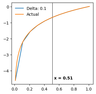
Setting \(x=0.51\)

\begin{equation} \frac{d}{dx}~ln(0.51) = 1.960784 ~~~~~~~~ \frac{d^2}{dx^2}~ln(0.51) = -3.844675 \end{equation} ### Plots with the numerical vs. actual values

gen_plot(3, [0.1], 0.51, 10)

Numerical first derivative for delta of 0.1

derivs_1d = []
for d, delta in enumerate([0.1]):
    df = do_derivs(delta, base=0.51, steps=10)
    df['index'] = d
    derivs_1d.append(df)
derivs_1d = pd.concat(derivs_1d, axis=1).T
derivs_1d['index'] = derivs_1d['index'].astype(int)
derivs_1d

	actual	delta	two-point	four-point	six-point	eight-point	index
0	1.960784	0.1	1.986509	1.958101	1.961712	1.959824	0

Numerical second derivative for delta of 0.1

derivs_2d = []
for d, delta in enumerate([0.1]):
    df = do_derivs(delta, base=0.51, steps=10, first=False)
    df['index'] = d
    derivs_2d.append(df)
derivs_2d = pd.concat(derivs_2d, axis=1).T
derivs_2d['index'] = derivs_2d['index'].astype(int)
derivs_2d

	actual	delta	two-point	four-point	six-point	eight-point	index
0	-3.844675	0.1	-3.920533	-3.835843	-3.847904	-3.841204	0