Analysis of James Bond franchise movies

This is a small notebook where I am doing some small analysis on the movies from the James Bond franchise. I am using ratings data from the MovieLens data set recommended for education and development, hand-copied data from The Numbers Movie Franchises for the budget, release dates, and total earnings. I am also using the IMDb ratings data set for comparison to the MovieLens data set.

This was actually prompted by trying to analyze different franchises and I saw that horror movie franchises are actually really profitable and it made me curious as to what other movie franchises have. I then saw that the James Bond franshise had a lot of the early movies be quite profitable (high return on investment) and I started to dig a bit deeper and it turned into this notebook where I try to find a reason why with the data that I have available to me.

I hope you enjoy going through this notebook as much as it was for me to create it all and learn a lot more about how pandas can be used in data manipulation and how dataframes are joined together like in SQL.

Imports and function definitions

from matplotlib.lines import Line2D
import ipywidgets as widgets
import matplotlib.pyplot as plt
import pandas as pd
import numpy as np
import os

def get_roi(data):
    '''
    Get the return on investment for the data set

    Args:
        data (pandas.DataFrame): Data frame with the budget
            and earnings data.

    Returns:
        df (pandas.DataFrame): Data frame copied from the
            original data with two new columns 'profit' and
            'roi'.
    '''
    df = data.copy()
    df['profit'] = df['earningsTotal'] - df['budgetTotal']
    df['roi'] = df['profit'] / df['budgetTotal'] * 100
    return df

def align_y_axis(ax1, ax2):
    '''
    Align two matplolib.axes.Axes objects such that the
    0's on the y-axis of the plots are aligned correctly.
    This function works such that the plots are zoomed out
    by a ratio that will force the 0's to align.

    Args:
        ax1 (matplotlib.axes.Axes): Axes object from the
            plot.
        ax2 (maptlotlib.axes.Axes): Axes object from the
            plot. Typically a twinx object.
    '''
    axes = (ax1, ax2)
    extrema = [ax.get_ylim() for ax in axes]
    tops = [extr[1] / (extr[1] - extr[0]) for extr in extrema]
    if tops[0] > tops[1]:
        axes, extrema, tops = [list(reversed(l)) for l in (axes, extrema, tops)]
    tot_span = tops[1] + 1 - tops[0]
    b_new_t = extrema[0][0] + tot_span * (extrema[0][1] - extrema[0][0])
    t_new_b = extrema[1][1] - tot_span * (extrema[1][1] - extrema[1][0])
    axes[0].set_ylim(extrema[0][0], b_new_t)
    axes[1].set_ylim(t_new_b, extrema[1][1])

def get_name(df, column):
    ''' Just a small helper function '''
    name = df[column].unique()
    if name.shape[0] > 1:
        raise ValueError("Failed determining name for column {}".format(column))
    else:
        name = name[0]
    return name

def get_actorName(actorId):
    actors = data_df['franchise_tags'][['actor', 'actorId']].drop_duplicates() \
                .set_index('actorId').T.to_dict(orient='list')
    try:
        actorName = actors[actorId][0]
    except KeyError:
        raise KeyError('There is no actor with an actorId value of {}'.format(actorId))
    return actorName

def get_movieName(movieId):
    movies = jb_ratings[['title', 'movieId']].drop_duplicates() \
                .set_index('movieId').T.to_dict(orient='list')
    try:
        movieName = movies[movieId][0]
    except KeyError:
        raise KeyError('There is no movie with the movieId value of {}'.format(movieId))
    return movieName

def get_movieDate(movieId):
    movies = jb_ratings[['date', 'movieId']].drop_duplicates() \
                .set_index('movieId').T.to_dict(orient='list')
    try:
        movieDate = movies[movieId][0]
    except KeyError:
        raise KeyError('There is no movie with the movieId value of {}'.format(movieId))
    return movieDate

def get_actorId(actorName):
    actors = data_df['franchise_tags'][['actor', 'actorId']].drop_duplicates() \
                .set_index('actor').T.to_dict(orient='list')
    try:
        actorId = actors[actorName][0]
    except KeyError:
        raise KeyError('There is no actor with the name {}'.format(actorName))
    return actorId

def generate_ratings(actorName, df, fstart):
    '''
    Generate a plot figure for the ratings of the specific
    actor given as an input. It is hard-coded that it will
    get the average rating over a yearly period.

    Args:
        actorName (str): Name of the actor for which you
            want to generate the plot.

    Returns:
        fig (matplotlib.pyplot.figure): Matplotlib figure
            object with the plotted data.
    '''
    actorId = get_actorId(actorName)
    label = '{:s} ({:d})'
    data = df.groupby('actorId').get_group(actorId)
    fig = plt.figure(fstart+actorId, figsize=(10,5), dpi=75)
    ax = fig.add_subplot(111)
    for movieId, sub_data in data.groupby('movieId'):
        movieName = get_name(sub_data, 'title')
        releaseDate = get_name(sub_data, 'date')
        all_time_avg = sub_data['rating'].mean()
        tmp = sub_data.groupby(pd.Grouper(key='reviewDate', freq='1Y'))['rating'].mean()
        ax.plot(tmp.index, tmp, label=label.format(movieName, releaseDate.year))
    ax.set_title(actorName, fontsize=18)
    ax.legend(bbox_to_anchor=(1.01,1), loc='upper left',
              fontsize=14)
    fig.tight_layout()
    return fig

def generate_hist(actorName, df, fstart):
    '''
    Generate a histogram plot of the ratings for each movie
    of the specific actor given as an input. Will display
    the mean, standard deviation, and total votes in the plot
    title. We also add the probability density with the
    parameters as calculated by the matplotlib histogram
    method. The plot will be displayed as the probability
    density instead of the total number of votes for the bin.

    Args:
        actorName (str): Name of the actor for which you
            want to generate the plot.

    Returns:
        fig (matplotlib.pyplot.figure): Matplotlib figure
            object with the plotted data.
    '''
    actorId = get_actorId(actorName)
    data = df.groupby('actorId').get_group(actorId)
    label = '{name:s} ({date:d})\navg: {avg:.2f} | std: {std:.2f}' \
            +'\nmedian: {med:.2f} | votes: {nvotes:d}'
    nrows = int(np.ceil(data['movieId'].unique().shape[0]/2))
    fig = plt.figure(fstart+actorId, figsize=(10,nrows*4), dpi=75)
    for idx, (movieId, sub_data) in enumerate(data.groupby('movieId')):
        ax = fig.add_subplot(nrows,2,idx+1)
        movieName = get_name(sub_data, 'title')
        releaseDate = get_name(sub_data, 'date')
        all_time_avg = sub_data['rating'].mean()
        all_time_median = sub_data['rating'].median()
        nvotes = sub_data.shape[0]
        hist_data = np.histogram(sub_data['rating'], bins=10, range=[0,5])
        n, bins, patches = ax.hist(sub_data['rating'], bins=10, range=[0,5],
                                   width=0.4, align='mid', density=True)
        # add a 'best fit' line
        sigma = sub_data['rating'].std()
        mu = all_time_avg
        y = ((1 / (np.sqrt(2 * np.pi) * sigma)) *
             np.exp(-0.5 * (1 / sigma * (bins - mu))**2))
        ax.plot(bins, y, '--')
        ax.axvline(all_time_avg, color='k', linestyle='-')
        ax.axvline(all_time_median, color='k', linestyle=(0, (5, 6)))
        kwargs = dict(name=movieName, date=releaseDate.year, avg=all_time_avg,
                      med=all_time_median, std=sigma, nvotes=nvotes)
        ax.set_title(label.format(**kwargs), fontsize=18)
    fig.suptitle('Histogram of ratings with {} as lead actor'.format(actorName), fontsize=24)
    fig.tight_layout(rect=(0,0,1,0.99))
    return fig

def generate_lineplot(actorName, df, fstart):
    # print(df)
    actorId = get_actorId(actorName)
    data = df.groupby('actorId').get_group(actorId)
    nrows = int(np.ceil(data['movieId'].unique().shape[0]/2))
    fig = plt.figure(fstart+actorId, figsize=(10,nrows*4), dpi=75)
    for idx, (movieId, sub_data) in enumerate(data.groupby('movieId')):
        ax = fig.add_subplot(nrows,2,idx+1)
        ax1 = ax.twinx()
        orig = sub_data.groupby('type').get_group('original')
        sub_data.drop(orig.index, inplace=True)
        movieName = get_movieName(movieId)
        movieDate = get_movieDate(movieId)
        xticks = [x+' ('+str(y)+')' for x, y in zip(sub_data['type'], sub_data['count'])]
        ax.plot(xticks, sub_data['average'], label='Average', color='tab:blue',
                marker='o')
        ax.plot(xticks, sub_data['median'], label='Median', color='tab:orange',
                marker='o')
        ax1.plot(xticks, sub_data['std'], color='tab:green', label='STD',
                marker='o')
        ax.axhline(orig['average'].values[0], color='tab:blue', linestyle=(0, (5, 6)))
        ax.axhline(orig['median'].values[0], color='tab:orange', linestyle=(0, (5, 6)))
        ax1.axhline(orig['std'].values[0], color='tab:green', linestyle=(0, (5, 6)))
        h1, l1 = ax.get_legend_handles_labels()
        h2, l2 = ax1.get_legend_handles_labels()
        custom = [Line2D([0], [0], color='k', linestyle='--')]
        handles = h1+h2+custom
        labels = l1+l2+['Original']
        ax.legend(handles, labels, bbox_to_anchor=(1.15,1), loc='upper left')
        ax.set_ylabel('Rating / out of 5')
        ax1.set_ylabel('STD')
        ax.set_title('{:s} ({:d})'.format(movieName, movieDate.year))
        for label in ax.get_xticklabels():
            label.set_rotation(40)
            label.set_horizontalalignment('right')
    fig.tight_layout()
    return fig

def gen_tab_object(func, df, fstart):
    names = ['Daniel Craig', 'Pierce Brosnan', 'Roger Moore', 'Sean Connery',
         'Timothy Dalton', 'George Lazenby', 'David Niven']
    out1 = widgets.Output()
    out2 = widgets.Output()
    out3 = widgets.Output()
    out4 = widgets.Output()
    out5 = widgets.Output()
    out6 = widgets.Output()
    out7 = widgets.Output()
    with out1: plt.show(func('Daniel Craig', df=df, fstart=fstart))
    with out2: plt.show(func('Pierce Brosnan', df=df, fstart=fstart))
    with out3: plt.show(func('Roger Moore', df=df, fstart=fstart))
    with out4: plt.show(func('Sean Connery', df=df, fstart=fstart))
    with out5: plt.show(func('Timothy Dalton', df=df, fstart=fstart))
    with out6: plt.show(func('George Lazenby', df=df, fstart=fstart))
    with out7: plt.show(func('David Niven', df=df, fstart=fstart))
    tabs = widgets.Tab(children=[out1, out2, out3, out4, out5, out6, out7])
    [tabs.set_title(i, name) for i, name in enumerate(names)]
    return tabs

Parse the data

dfs = {}
dirs = dict(large='ml-latest')
files = ['franchise_movies.csv', 'franchise_tags.csv', 'links.csv', 'ratings.csv']
for key, parent in dirs.items():
    dfs[key] = {}
    for fn in os.listdir(parent):
        if not fn.endswith('.csv'): continue
        if fn not in files: continue
        sub_key = fn.replace('.csv', '')
        dtypes = dict(userId=int, movieId=int,
                      imdbId=str, tmdbId=str)
        filename = os.path.join(parent, fn)
        dfs[key][sub_key] = pd.read_csv(filename, dtype=dtypes)
all_data = dfs

main = 'imdb-data'
parent = 'title-ratings'
dtypes = dict(tconst=str, numVotes=int)
fn = os.path.join(main, parent, 'data.tsv')
df = pd.read_csv(fn, sep='\t', dtype=dtypes)
df['tconst'] = df['tconst'].apply(lambda x: x[2:])
df = df.merge(all_data['large']['links'], left_on='tconst', right_on='imdbId', how='right')
all_data['imdb-ratings'] = df

Convert timestamps to human readable dates

data_df = all_data['large'].copy()
data_df['franchise_movies']['date'] = pd.to_datetime(data_df['franchise_movies']['releaseDate'], unit='s')

Analysis of return on investment

indv_roi = get_roi(data_df['franchise_movies'])

jb_movies = indv_roi.groupby('seriesId').get_group(10).copy()
jb_movies['date'] = pd.to_datetime(jb_movies['releaseDate'], unit='s')
jb_movies.sort_values(by=['roi'], ascending=False)[['title', 'date', 'budgetTotal', 'profit', 'roi']].reset_index(drop=True)

	title	date	budgetTotal	profit	roi
0	Dr. No	1963-05-08	1000000	58567035	5856.703500
1	Goldfinger	1964-12-22	3000000	121900000	4063.333333
2	From Russia with Love	1964-04-08	2000000	76900000	3845.000000
3	Live and Let Die	1973-06-27	7000000	154800000	2211.428571
4	Diamonds Are Forever	1971-12-17	7200000	108799985	1511.110903
5	Thunderball	1965-12-29	9000000	132200000	1468.888889
6	The Man with the Golden Gun	1974-12-20	7000000	90600000	1294.285714
7	The Spy Who Loved Me	1977-07-13	14000000	171400000	1224.285714
8	You Only Live Twice	1967-06-13	9500000	102100000	1074.736842
9	On Her Majesty's Secret Service	1969-12-18	8000000	74000000	925.000000
10	For Your Eyes Only	1981-06-26	28000000	167300000	597.500000
11	Octopussy	1983-06-10	27500000	160000000	581.818182
12	Moonraker	1979-06-29	31000000	179300000	578.387097
13	Goldeneye	1995-11-17	60000000	296429933	494.049888
14	Casino Royale	2006-11-17	102000000	492420216	482.764918
15	Skyfall	2012-11-08	200000000	910526981	455.263490
16	A View to a Kill	1985-05-24	30000000	122627960	408.759867
17	The Living Daylights	1987-07-31	40000000	151199996	377.999990
18	Never Say Never Again	1983-10-07	36000000	124000000	344.444444
19	Licence to Kill	1989-07-14	42000000	114167015	271.826226
20	Casino Royale	1967-04-28	12000000	29744718	247.872650
21	Tomorrow Never Dies	1997-12-19	110000000	229504276	208.640251
22	Die Another Day	2002-11-22	142000000	289942139	204.184605
23	No Time to Die	2021-10-08	250000000	509959662	203.983865
24	Spectre	2015-11-06	300000000	579077344	193.025781
25	The World is Not Enough	1999-11-19	135000000	226730660	167.948637
26	Quantum of Solace	2008-11-14	230000000	361692078	157.257425

What you can actually see is that a lot of the older James Bond movies actually have a much higher return on investment that the newer ones with Quantum of Solace actually performing the worst. Could this stem from how action movies themselves are more expensive to produce?

fig = plt.figure(1, figsize=(6,6), dpi=75)
x = np.linspace(jb_movies['releaseDate'].min(), jb_movies['releaseDate'].max(), 100)
ax = fig.add_subplot(111)
ax2 = ax.twinx()
ax.axhline(0, color='k', linewidth=0.7)
ax.plot(jb_movies['date'], jb_movies['roi'], 'o', label='Return on Investment')
ax2.plot(jb_movies['date'], jb_movies['profit']/1e6, '^', color='tab:red', label='Profit')
ax.set_xlabel('Date')
ax.set_ylabel('Return on investment / %')
ax2.set_ylabel('Profit (not adjusted for inflation) / 10$^6$ USD')
ax.set_title('Return on investment for James Bond movies')
h1, l1 = ax.get_legend_handles_labels()
h2, l2 = ax2.get_legend_handles_labels()
handles = h1 + h2
labels = l1 + l2
ax.legend(handles, labels, bbox_to_anchor=(1.01,1), loc='upper left')
align_y_axis(ax, ax2)

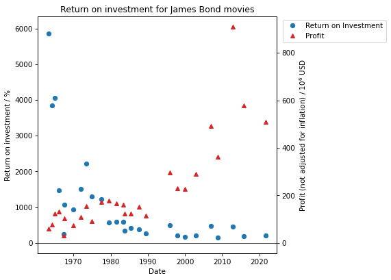
Here we see a plot of the return on investment for the James Bond series in blue and the profit in red. We see how the profit (not adjusted for inflation) actually goes up significantly. So let’s maybe take a look at how the ratings for the movies has changed over time.

Ratings per lead actor

df1 = jb_movies.copy()
df1.reset_index(drop=True, inplace=True)
tmp = data_df['ratings'].merge(df1[['movieId', 'title', 'releaseDate', 'date', 'roi']], on='movieId')
jb_ratings = tmp.merge(data_df['franchise_tags'][['movieId', 'actor', 'actorId']], on='movieId')
jb_ratings['reviewDate'] = pd.to_datetime(jb_ratings['timestamp'], unit='s')

tabs = gen_tab_object(generate_ratings, jb_ratings, 2)
tabs

Unfortunately, our dataset that we got from MovieLens is incomplete for all but the James Bond movies starring Daniel Craig and Pierce Brosnan as they are just too old. Overall, however, there does not seem to be a consistent trend in the data showing a reason for either a decrease or increase of return on investment or profit, respectively.

A quick look through Wikipedia ( this in particular) actually shows a steady increase in the salary of the lead actors and if we factor the increased use of VFX and stunts it might be enough to really show how the movies don’t have as big of a return on investment, and with an increased use of VFX and the advancement in the realism of VFX could be a contributing factor to the increase in profits over time.

One last thing that I wanted to look at is the stability of the data. I.e. how does the data we used above really compare with other datasets. I will compare the average ratings to those from IMDb and see how far from the median the average is.

Comparing to IMDb data

grouped = jb_ratings.groupby('movieId')
count = grouped['rating'].count().rename('count')
all_time_avg = grouped['rating'].mean().rename('average')
all_time_median = grouped['rating'].median().rename('median')
all_time_std = grouped['rating'].std().rename('std')
df = pd.concat([all_time_avg, all_time_median, all_time_std, count], axis=1)
df = df.merge(all_data['imdb-ratings'][['averageRating', 'numVotes', 'movieId']], on='movieId')
df = df.merge(jb_movies[['title', 'movieId', 'date']], on='movieId')
df['title'] = df['title'] + df['date'].apply(lambda x: ' ('+str(x.year)+')')
df['averageRating'] /= 2
df['numVotes'] = df['numVotes'].astype(int)
rcols = dict(averageRating='imdbRating', numVotes='imdbVotes')
df.rename(columns=rcols).set_index('title').sort_values(by=['date']).drop(['movieId', 'date'], axis=1)

	average	median	std	count	imdbRating	imdbVotes
title
Dr. No (1963)	3.665154	4.00	0.835024	9694	3.60	175470
From Russia with Love (1964)	3.688400	4.00	0.849023	9586	3.65	141772
Goldfinger (1964)	3.729858	4.00	0.865900	15527	3.85	198327
Thunderball (1965)	3.599912	3.50	0.846492	5690	3.45	124284
Casino Royale (1967)	2.877232	3.00	1.054743	1120	2.50	31603
You Only Live Twice (1967)	3.593695	3.50	0.802609	3394	3.40	114921
On Her Majesty's Secret Service (1969)	3.428017	3.50	0.932231	3605	3.35	96895
Diamonds Are Forever (1971)	3.495077	3.50	0.852021	5992	3.25	111678
Live and Let Die (1973)	3.488243	3.50	0.857393	6294	3.35	112948
The Man with the Golden Gun (1974)	3.464959	3.50	0.852398	5037	3.35	110691
The Spy Who Loved Me (1977)	3.531111	3.50	0.840140	5609	3.50	113778
Moonraker (1979)	3.158547	3.00	0.939335	6014	3.10	106341
For Your Eyes Only (1981)	3.437548	3.50	0.868478	5212	3.35	106002
Octopussy (1983)	3.310463	3.50	0.881729	2332	3.25	110735
Never Say Never Again (1983)	3.266388	3.50	0.931870	1556	3.05	71465
A View to a Kill (1985)	3.182722	3.00	0.920832	4526	3.15	102587
The Living Daylights (1987)	3.290004	3.00	0.890285	2731	3.35	103645
Licence to Kill (1989)	2.625000	2.75	1.187735	8	2.75	1028
Goldeneye (1995)	3.434835	3.50	0.878003	34942	3.60	265904
Tomorrow Never Dies (1997)	3.230008	3.00	0.935325	15919	3.25	201493
The World is Not Enough (1999)	3.204092	3.00	0.952916	11583	3.20	206889
Die Another Day (2002)	3.086181	3.00	0.999052	8720	3.05	225752
Casino Royale (2006)	3.837693	4.00	0.862241	28517	4.00	680473
Quantum of Solace (2008)	3.300951	3.50	0.935187	10196	3.30	463211
Skyfall (2012)	3.741676	4.00	0.890015	15918	3.90	718361
Spectre (2015)	3.392451	3.50	0.936909	5630	3.40	457116
No Time to Die (2021)	3.484932	3.50	0.884875	1626	3.65	430310

The overall conclusion from this is that the data from MovieLens seems to not have a large skew, albeit having a smaller sample size than IMDb with the exception of Licence to Kill (1989) which only has 8 votes and that is reflected in the larger standard deviation to the rest. It would be interesting to see how the standard deviation and median compare for the IMDb data, but I don’t have access to that data, unfortunately.

See how normalized the ratings are

Something else that we could look at to see how the data is actually behaving is to look at how close to the average the individual data points are. So we will plot the votes into a histogram and see how nice of a bell-curve it makes.

tabs = gen_tab_object(generate_hist, jb_ratings, 9)
tabs

Note: Average is represented by the solid black line and the median is the dashed black line.

What we can actually see here is that for most of the plots the maximum in the probability density distribution function lines up pretty well with the bins with the highest number of votes. However, for movies starring Daniel Craig, the distribution is very even, whereas for movies starring someone like Pierce Brosnan there are some peaks and valleys in the data for movies like Goldeneye (1995) which seems to be the most popular one with the highest number of votes out of any other James Bond film. This does not necessarily point to any issues with the dataset, however, I am wondering if there might be some kind of bias towards whole numbers from those voting. This seems to also be a trend is some of the other movies with Roger Moore and Sean Connery as James Bond.

Comparison of voting with different kinds of viewers

Here I just want to look at differences in voting for people that are casual watchers and fans. I am using the following definitions

• casual: people that have voted for less than 2 movies inclusive

• story fans: people that voted for at least 3 movies but less than 8 movies

• super story fans: people that voted for at least 8 movies

• godly fans: people that have voted for at least 16 movies

• super godly fans: people that have voted for at least 20 movies

df = jb_ratings.copy()
count = df.groupby('userId')['rating'].count().rename('count')

Casual group

ids = count[count <= 2]
casual_df = df.merge(ids, on='userId', how='right')

tabs = gen_tab_object(generate_hist, casual_df, 9)
tabs

Story fans group

ids = count[count.between(3, 7)]
stfans_df = df.merge(ids, on='userId', how='right')

tabs = gen_tab_object(generate_hist, stfans_df, 9)
tabs

Super story fans group

ids = count[count.between(8, 15)]
spstfans_df = df.merge(ids, on='userId', how='right')

tabs = gen_tab_object(generate_hist, spstfans_df, 9)
tabs

Godly fans group

ids = count[count >= 16]
godfans_df = df.merge(ids, on='userId', how='right')

tabs = gen_tab_object(generate_hist, godfans_df, 9)
tabs

Super Godly fans group

ids = count[count >= 22]
spgodfans_df = df.merge(ids, on='userId', how='right')

tabs = gen_tab_object(generate_hist, spgodfans_df, 9)
tabs

Based on what we see here, the distributions seem to become a bit more normalized and don’t seem to favor integer numbers for the ratings. This does not necessarily mean that the data is better than before because now there may be a bias as some of the groups, like super godly, are made of people that have watched many James Bond movies and may no longer represent the general public.

Putting it all together

Here I will compile all of the data from above and try to make a solid judgement.

dfs = {'original': jb_ratings, 'casual': casual_df, 'story': stfans_df,
       'super story': spstfans_df, 'godly': godfans_df,
       'super godly': spgodfans_df}
arr = []
for key, val in dfs.items():
    grouped = val.groupby(['actorId', 'movieId'])
    avg = grouped['rating'].mean().rename('average')
    med = grouped['rating'].median().rename('median')
    std = grouped['rating'].std().rename('std')
    cnt = grouped['rating'].count().rename('count')
    df = pd.concat([avg, med, std, cnt], axis=1)
    df['type'] = key
    df.reset_index(inplace=True)
    arr.append(df)
df = pd.concat(arr, ignore_index=True)
combined_df = df

tabs = gen_tab_object(generate_lineplot, combined_df, 9)
tabs

Here we see that for the most part limiting those who voted to the criteria that I outlined before does not seem to have as big of an effect as I originally thought. However, we do see that the standard deviation does decrease for some movies and for others there does not seem to be any improvement. This is not supposed to say that the people that have watched more James Bond movies make a “better” reviewer. It is just to say that some of the users that have watched more James Bond movies may look for different things in the movie as opposed to those that do not watch them as much. Some things could include the story, visual effects, action sequences, villains, to name a few.

Conclusion

I am happy to claim that the dataset that I am using, while is not necessarily the largest as there are only 8 votes for Licence to Kill (1989), does have similar ratings to those from IMDb and the median values are not that far off the average. In addition, the distribution of the votes seems pretty normalized. Finally, we tried to see how the number of James Bond movies would affect the averages, medians, and standard deviations, where there was not a large dependence on it. However, the distributions seem a bit more normalized and not favoring integer numbers for the ratings. However, by grouping the users like this it may no longer be a good description of the entire population as it is adding a bias to the results. It is, however, interesting to see this trend.

So, based on the data I have I cannot make a conclusion on what has caused the huge decrease in the return on investment for James Bond movies over the years. Only when I went to Wikipedia and did some manual digging did I come across something that could be a factor, salary of the lead actors.

Thank you for coming along with me on this fun journey!!